
Classifying Publicly Available LiDAR Data with Deep Learning
Will this even be useful?

In my previous article, I spoke about 3D modeling using LiDAR data and the various deep learning packages Esri provides. I mentioned how data is usually the most difficult thing to come by, and how the Microsoft Planetary Computer has an extensive catalog of LiDAR data. We were left with this question:
Has the public availability of data and tools really made geospatial AI processes available to everyone?
We’ll go about answering that question by reviewing how the data was acquired, prepared, and classified. Our study area is the town I live in: Hermiston, Oregon.
Acquiring the Data
If you recall, the data catalog in the Microsoft Planetary Computer includes some LiDAR point clouds, listed under the DEM topic. If you are unfamiliar with a DEM (digital elevation model), it is probably something you’ve probably seen before without realizing it.
Try going to google maps, clicking the Layers square button on the screen, and switching from imagery to map.
In the series of buttons next to it, toggle the “Terrain” button off and on a few times. See the below video for a demonstration.
That terrain layer which shows a kind of shadowing around higher elevation areas really adds definition to the map. That’s a DEM—a 3D representation of the Earth’s surface.
One of the ways to make a DEM is with a LiDAR point cloud. We’re not interested in making a DEM per se in the context of this article—to do so, you would need to clear away all the non-ground data that a LiDAR point cloud contains within it—anything hitting buildings, trees, or other structures are not part of a DEM. Including those items has its own name - a DSM, or Digital Surface Model. Both models have value, but they are different things.
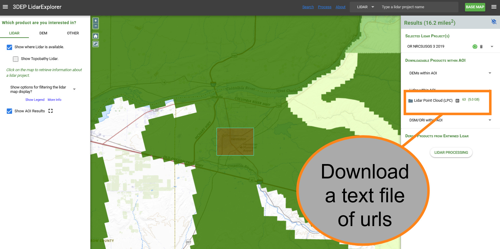
The LiDAR point cloud I used in the Microsoft Planetary Computer catalog comes from the USGS (U.S. Geological Survey) 3DEP program, also known as the 3D Elevation program. The program has elevation data for over 98% of the land area of the United States. The data is available through the 3DEP LiDAR Explorer. As you might expect, the data comes with the ground already classified—it’s use in 3DEP is apparently mostly concerned with elevation. But the raw point cloud should contain the other data as well.
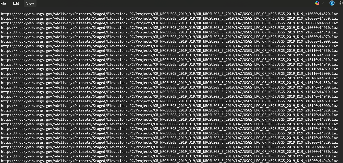
Using the LiDAR Explorer was straightforward. You could draw a rectangle around your area of interest and search for point clouds in that area. The coverage for an individual point cloud is rather small, likely because larger point clouds would become prohibitively large in size, especially on the web. If you’re interested in a small area, you might just download those point clouds using the Explorer. For our purposes however, we are trying to model a large portion of the city of Hermiston, which equates to about 58 point cloud files. For that, I chose to download a text file of url download links. If you were to copy a single url and paste it into your browser, it would begin downloading that file immediately.
I had no desire to go through the process 58 times. I know a bit of the scripting language python, so I chose to use those skills to automate the process. For each line in the text document, the script would open it and download the file. This took some doing—python doesn’t have the benefit of a browser to tell it to download a file—without that additional context, the url is just a series of characters. To do this, I had to import a python library called urllib.1
Processing the Data
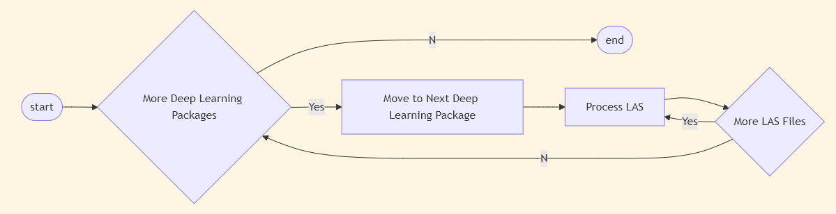
Before we get into the processing steps, let’s review what we’re doing here: We’re evaluating the Esri deep learning packages against publicly available and easy-to-retrieve LiDAR data. The chart below shows the steps taken to go from step A to step Z, but that is with the benefit of hindsight. As an exploratory process, all I really knew at the beginning was that I was going to download the data, and apply the Power Lines deep learning package to it (I also ended up adding Buildings and Trees to the mix)
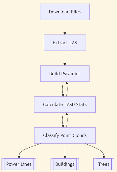
There were a few things that I learned along the way in terms of the data processing flow, and I’ll outline them here:
Files in the Wrong Format
The files download as LAZ, but ArcGIS Pro and the deep learning packages need LAS files. LAZ is a compressed version of an LAS, so these files are likely being saved in that format to save space—the LAZ files I downloaded took up 4.3GB of space, but the LAS files I ended up with took up over 24GB.
Draw Speeds Very Slow
Once the data is loaded up into ArcGIS Pro, it is excruciatingly slow. I’ve done enough geospatial data processing to know this is probably due to some steps I needed to take to speed things up a bit—which ended up being building pyramids and calculating statistics, which we’ll get into later.
Utilizing the LAS Dataset
In ArcGIS Pro and through python scripts you could load up each individual LAS, or you could create an LAS dataset, which acts as a sort of index. You add the dataset file, and it automatically includes all the associated LAS files. This sped things up and simplified them for the most part, but doing data processing using the LAS Dataset file was problematic, simply because my computer didn’t like trying to process that much data all at once.
Step 1: Extract LAS
What is the first thing you do when you download some cool LiDAR data? Open it in your application of choice of course—in my case, ArcGIS Pro. I quickly found out that the LAZ file is persona non-grata and needs to be converted first using the Extract LAS (3D Analyst) tool.
There are likely some applications that can display LAZ files natively, however the LAZ file is a lossless compression format, meaning the data is compressed to keep the file sizes smaller. There is a trade-off to this: performance. A compressed format means applications have to do more work to show you the data, converting from that compressed format on the fly. LAS, on the other hand, is not compressed, and therefore not subject to the performance drawbacks of compression. I say all this to say that Esri has clearly made the calculation that displaying LAZ would be too slow, and therefore did not build into ArcGIS Pro the ability to read it—instead, we must convert it first.
Another benefit of the Extract LAS tool is the LAS Dataset, which can be created by running the tool. This dataset will take any number of LAS files and reference them, so that functionally on a map, you only see one layer of data, as opposed to a layer for each LAS—in our case, that would have been 58 separate layers. 58 layers to set display settings on, 58 layers to view in the table of contents. In this way, it acts as a sort of index. When I ran the Extract LAS tool, I created new LAS files from the 58 LAZ files and then create an LAS dataset file that referenced all 58 LAS files—this dataset layer is the one I would add to the map.2
Step 2: Pyramids and Statistics
As always, we remain concerned about performance. 58 separate files loading at once is quite the load on a computer. To solve this, we need to build pyramids with the Build LAS Dataset Pyramid tool—another benefit of the LAS Dataset. Here is Esri describing what the tool does in its documentation:
A LAS dataset pyramid structure is used to improve 3D display performance for a LAS dataset in ArcGIS Pro. It does this by organizing and indexing the points in a way that optimizes 3D display queries. LAS dataset pyramids use an octree-based indexing scheme that partitions space into a set of nested cubes. It's a 3D scheme that tends to retain more detail while still being fast. For example, an octree-based solution better supports visualizing and navigating to outlying points of a LAS dataset.
In other words, pyramids make the data display faster.
Another benefit of the LAS dataset is the ability to calculate statistics on the LiDAR data. We do this with the LAS Dataset Statistics (Data Management) tool. The tool creates spatial and attribute indexes for the data. Any database administrator will tell you that having up to date indexes is crucial for having an efficient and responsive database. Most production databases will calculate statistics on tables of data at set intervals: daily, weekly, etc. For an LAS file, the index is saved with the same name as the file, but with an LASX extension. Anytime the LAS file is altered (for example, classifying the data using one of the deep learning packages), statistics need to be recalculated to keep the data performant.3
Below I’ve included a short video, sped up, comparing the same data with pyramids and statistics calculated, and without. With the calculations, the model draws in 20 seconds. Without them, it draws in 2 minutes and 8 seconds—and didn’t even finish drawing all the way before the application gave up. Both layers are symbolized the same, but there are a few caveats to the below video—these are being run side by side on my PC and with other applications open, so as a test there are some other variables there, but you get the idea. Pyramids and statistics make a big difference in draw speed.
Another benefit of calculating statistics is the option to output the results to a table. I’ve included this table in the appendix for those interested.
Step 3: Classifying the Point Cloud
Finally, we’re at the money step! We’re going to use the Esri geoprocessing tool Classify Point Cloud Using Trained Model (3D Analyst). But before we do, we have to install the deep learning frameworks for ArcGIS on our PC. ArcGIS Pro (and the arcpy python library) do not come with this framework by default. Nevertheless, it is not difficult to install—think of it like installing a version of .NET or DirectX software that you might need. Once installed, it’s not something that you need to worry about until you upgrade ArcGIS Pro.
We also need the deep learning packages—in this case, the ones for power lines, buildings, and trees, which I downloaded and saved to my machine locally. They have a DLPK extension.
From there, it is a matter of running the tools for each deep learning package. The tool has settings that allow you to only classify those points which are not already classified, and this is a setting I used. From the statistics I ran earlier, I knew that running the tool only on unclassified points would work.
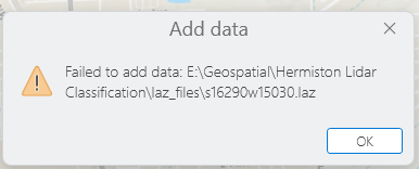
I started by running the tool on the LAS dataset—for those that don’t remember, this is the “index file” that references each LAS in the study area. This is a step that can probably done from within ArcGIS Pro, but since I had already started a python script, I decided to automate here as well. It failed pretty quickly, due to a memory error.
My computer is no slouch. It’s got a pretty new processor and has 32GB of RAM. But, it clearly had some trouble with this workload. So, I refactored my code to go through the LAS files directly—it grabbed each LAS in the directory (I had them all saved in the same place, ran the tool, then moved on. It also did this for each deep learning package. It looked something like this:
After running for several hours however, it would fail with the same memory error. My guess is the script was holding more information in memory than it needed to, because there is no reason for it to fail on an individual LAS. However, considering the time investment in running this script (I estimate it would take 10+ hours if it were to run start to finish without error), I instead decided to add in some logic to the script that would allow it to skip any LAS files that have already been processed. I continued on this way in a trial and error fashioned for a few days, until all three deep learning packages had run on all LAS files.
Results
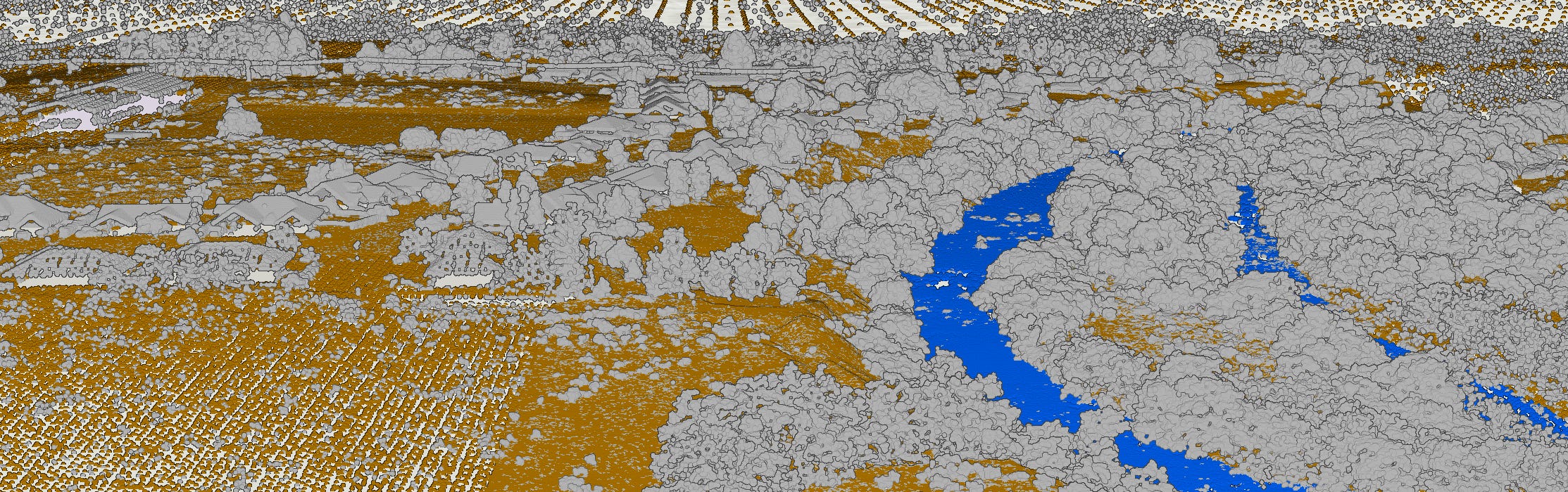
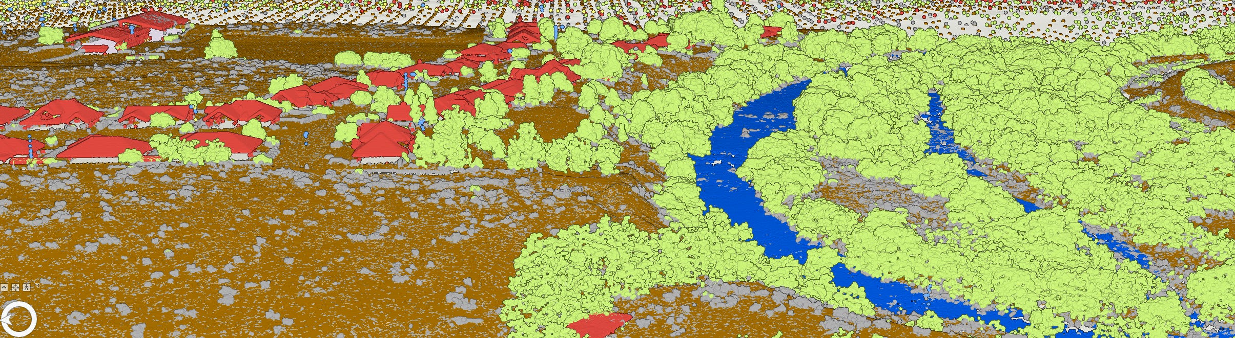
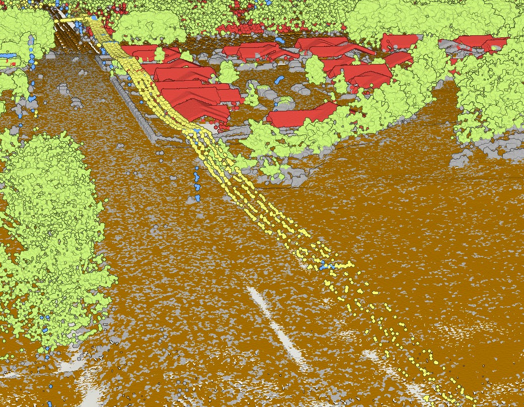
In addition to the tables in the Appendix, here are some screenshots that show the differences between the original LAS files, classified for ground and water, and the reclassified LAS files, including power lines, trees, and buildings:
Original
Reclassified Using Deep Learning Models
Which brings us back to our original question:
Has the public availability of data and tools really made geospatial AI processes available to everyone?
This probably depends how you think about it. I should note that this is run primarily with Esri tools using extensions that typically cost extra money—I am getting away with using a student edition of the software, but for a company trying to implement this sort of workflow, they are going to have to pony up for the licenses or else figure out how to do it with free, open source software.
Using these tools basically out of the box, they seem pretty effective at helping the user render something on the screen that looks pretty close to reality. But would this data stand up to a rigorous analysis workflow (especially in a way that makes it widely available on, say ArcGIS Online or some other Map Server)? In other words, can this data do more than just look pretty in ArcGIS Pro after running the deep learning tools? This remains to be seen. Take a look at the tables in the appendix. While we’ve cut the number of unclassified points in half, 11% of the points in the area remain unclassified. Things like roads, low-lying shrubs, and cars.
These are questions I hope to explore in future articles here at the Geospatial Explorer.
Appendix
Hermiston-Area LiDAR Dataset Statistics-Before Classification
Hermiston-Area LiDAR Dataset Statistics-After Classification
The relevant code can be found in the downloadFiles function in the userDefinedFunctions.py file of my code repository.
Extracting the LAS files was done with the extractLAS user defined function in the userDefinedFunctions.py file of my code repository.
See the buildPyramid and lasdStatistics user-defined function in userDefinedFunctions.py and main.py, in my code repository